03 - Decision Trees

Decision tree

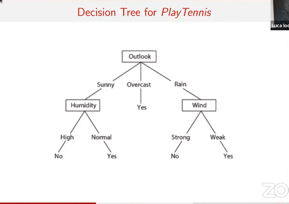
Tree with the following characteristics:

• each internal node tests an attribute $Ai$
• each branch is a value of an attribute $a_i,j\in A_i$
• each leaf node assigns a classification value $c\in C$
• a classic decision tree, like the ones in Algorithms

How to form a rule

• evaluates the branches we are interested in and put them in disjunction
• for example: IF (Outlook = Sunny) AND (Humidity = High) THEN PlayTennis = No

ID3 Algorithm

We have: INPUT: Examples (both positives and negatives), Target Attribute (Play Tennis), Attributes (Outlook, Wind…) OUTPUT: DT (Decison Tree)

We have three cases if attributes are empty:

1. Examples contains only positives: RETURN +
2. Examples contains only negatives: RETURN -
3. Both of them: + or -, depending on majority samples in D

(also called GENERAL CASE) We have these cases if attributes are NOT empty:

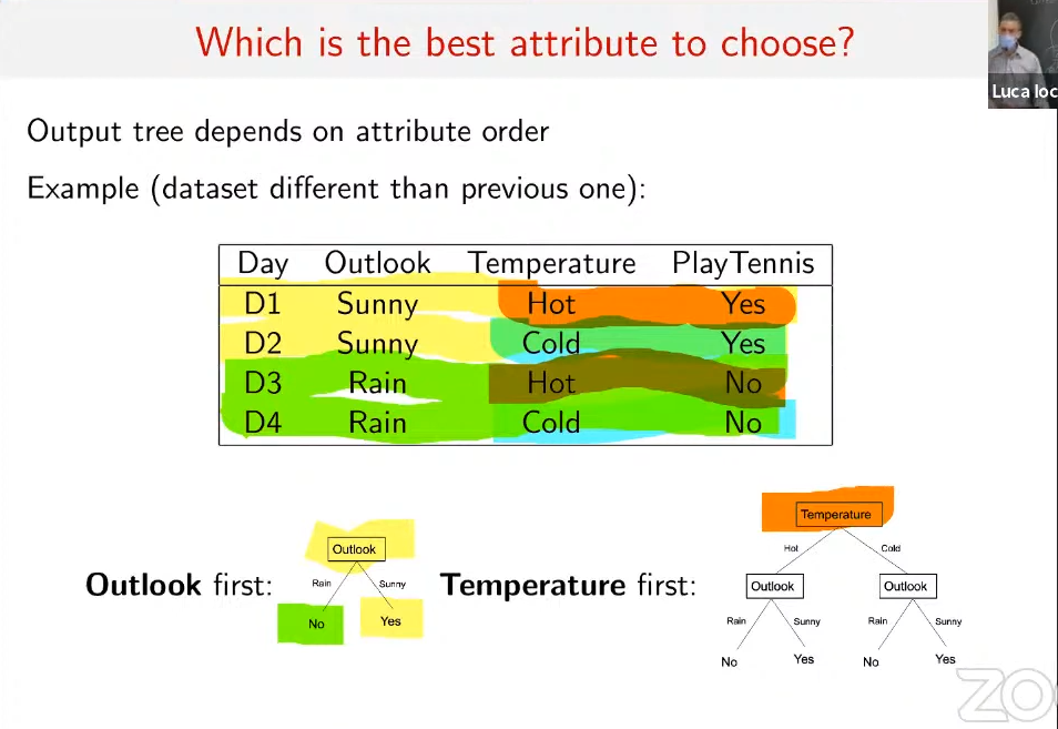
• let’s choose a specific attribute (by using a specific criteria)
• let’s create a node
• let’s create a child node
• let’s make a recursive call to build all the subsets
  • each recursive call will change the examples and the attributes EXCEPT the one I am already considering

An example is worth one thousand words:

Entropy and Information gain

it represents the impurity or randomness in a dataset $\text{Entropy}(S)=-{\sum }_{i=1}^n{p}_i{\log }_2(p_i)$

Information Gain measures the effectiveness of a feature in classifying a dataset. It quantifies how much information a feature provides about the class label. High information gain means a feature is very useful for classification.

To calculate information gain for a feature A with respect to a dataset S, you compute the entropy of the original dataset Entropy(S), and then calculate the weighted sum of entropies after splitting the dataset based on feature A. $\text{Information Gain}(S,A)=\text{Entropy}(S)-{\sum }_{v\in \text{Values}(A)}\frac{|S_v|}{|S|}\times \text{Entropy}(S_v)$

Example

Let’s consider a simple binary classification problem to illustrate how entropy and information gain are used in decision tree classification.

Suppose we have a dataset of emails that are classified as either spam (positive class) or non-spam (negative class). The dataset has two features:

1. Feature 1: Whether the email contains the word “lottery” (binary feature: 1 if yes, 0 if no).
2. Feature 2: Whether the email contains the word “discount” (binary feature: 1 if yes, 0 if no).

Let’s calculate entropy and information gain to decide the best feature for the first split in the decision tree.

Calculating Entropy for the Initial Dataset:

Let’s assume there are 60 emails in the dataset, with 30 being spam and 30 non-spam. $\text{Entropy}(S)=-\left(\frac{30}{60}{\log }_2\left(\frac{30}{60}\right)+\frac{30}{60}{\log }_2\left(\frac{30}{60}\right)\right)=-(0.5\times -1+0.5\times -1)=1$

Calculating Information Gain for Feature 1 (“lottery”):

Let’s assume 20 emails have the word “lottery” and 40 do not. $\text{Entropy}(S_{\text{lottery}})=-\left(\frac{10}{20}{\log }_2\left(\frac{10}{20}\right)+\frac{10}{20}{\log }_2\left(\frac{10}{20}\right)\right)=1$ $\text{Information Gain}(S,\text{lottery})=1-\left(\frac{20}{60}\times 1+\frac{40}{60}\times 1\right)=0$

Calculating Information Gain for Feature 2 (“discount”):

Let’s assume 25 emails have the word “discount” and 35 do not. $\text{Entropy}(S_{\text{discount}})=-\left(\frac{10}{25}{\log }_2\left(\frac{10}{25}\right)+\frac{15}{25}{\log }_2\left(\frac{15}{25}\right)\right)\approx 0.96$ $\text{Information Gain}(S,\text{discount})=1-\left(\frac{25}{60}\times 0.96+\frac{35}{60}\times 0.96\right)\approx 0.02$ In this example, Feature 2 (“discount”) has a higher information gain compared to Feature 1 (“lottery”). Therefore, the decision tree would choose “discount” as the first split, as it provides more information in reducing the uncertainty about the class labels.

So, entropy measures how mixed up things are, and information gain helps us figure out the best way to organize and understand the mix!

When the entropy is 0 all the subsets are such that in each subset there only are positives or negatives example!

ID3 for short

1. Create a rotto node
2. if all examples are pos, return Root with label +
3. if all examples are neg, return Root with label -
4. if attributes is empty, then return the node root with label = most common value of target_attribute in Examples
5. otherwise
   1. A ← the best decision attribute for Examples
   2. assign A as devision attribute for Root
      1. for each value $v_i$ of A
         • add a new branch from Root corresponding to the test A = $v_i$
         • $example{s}_{vi}$ = subset of Examples that have value $v_i$ for A
         • if $example{s}_{vi}$ is empty then add a leaf node with label = most common value of target_attribute in examples
         • else add the tree ID3($Example{s}_{vi}$, Target_attribute, Attributes-{A})

Avoid overfitting

• stop growing when data split not efficient
• grow full tree then post prune In pratica semplifichi un nodo mettendo al posto di un albero di decisione, un certo valore o meno.

GOOGLE COLAB HERE!